In short
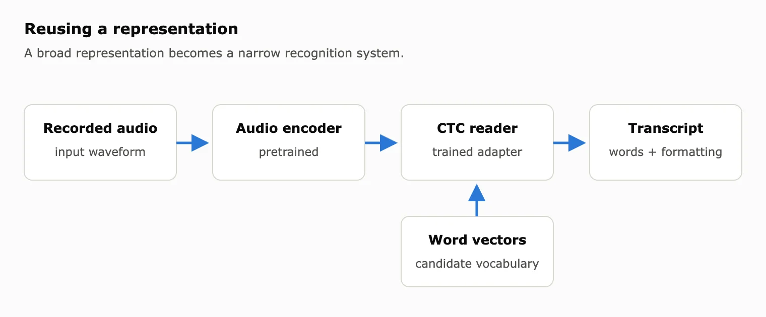
- Embedding Gemma Transcribe adapts a pretrained audio encoder with a CTC reader whose word targets use EmbeddingGemma’s text embeddings.
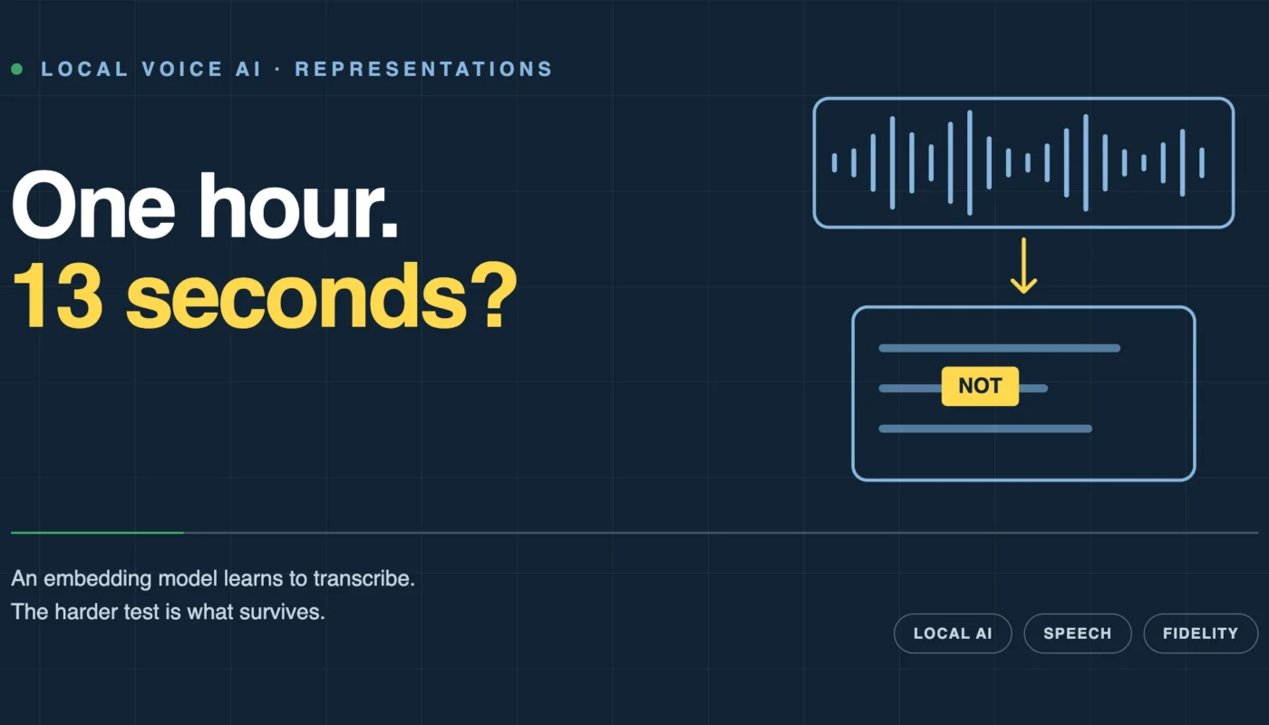
- The developer reports one hour transcribed in 12.6 seconds on an M3 MacBook Air. The timing is not a benchmark reproduced by Perit, and accuracy for that specific recording is not disclosed.
- Retrieval, exact transcription, and live conversation need different tests. Names, numbers, negation, partial transcripts, and turn timing each carry a separate obligation.
- Small specialists can make local AI practical. Their evaluation must cover the handoffs between recognition, formatting, turn detection, and speech synthesis.
An hour-long recording sits on a laptop. A progress bar moves, and the transcript appears before there is time to make coffee. The developer reports 12.6 seconds on a base M3 MacBook Air with 8 GB of RAM. The machine is ordinary. The recognizer has an unusual origin.
Embedding Gemma Transcribe adapts a model designed to represent information across different media. A pretrained audio encoder supplies the representation. A trained reader turns it into words. Another component adds punctuation and capitals. The headline is speed. The more interesting question is what that arrangement preserves.
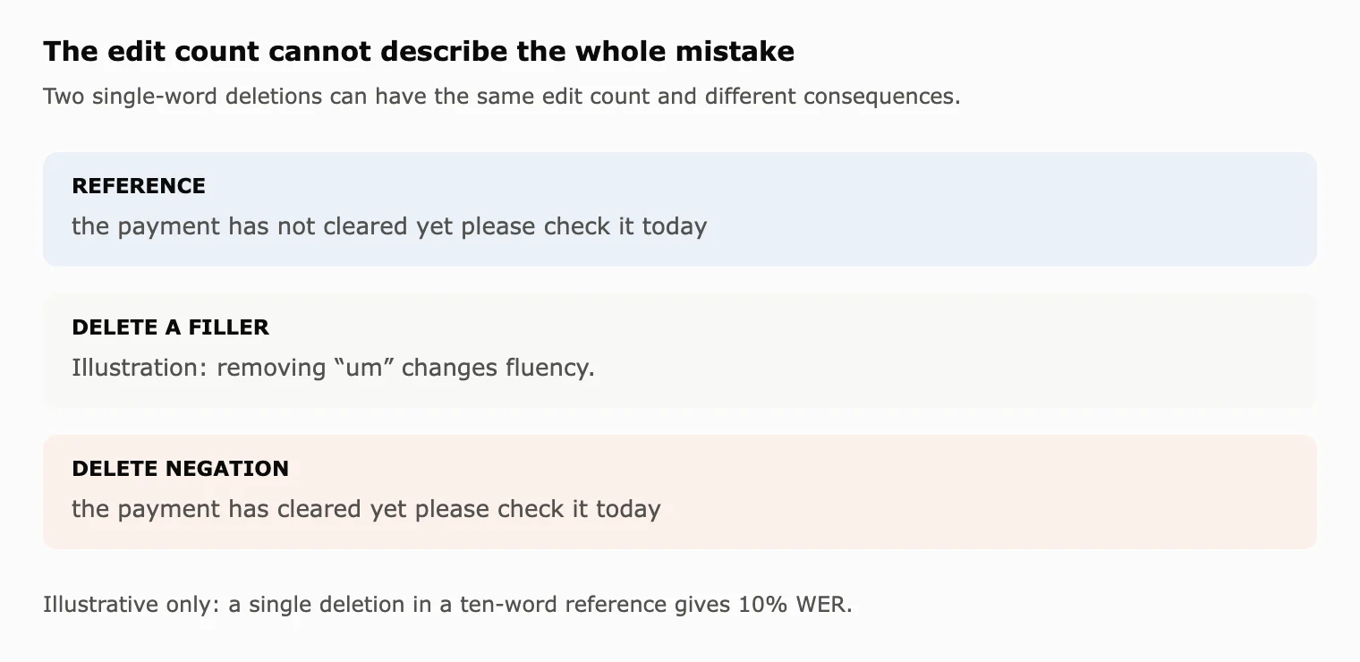
Consider an illustrative customer call: “The payment has not cleared. The reference is Kaira seventeen B.” Finding this call when someone searches for payment problems is useful. Writing “the payment has cleared” into a case record is disastrous. Both outputs concern the same topic. Only one preserves the instruction.
That gap carries the enterprise story. Local voice AI becomes valuable when a system can reuse broad capabilities while meeting narrow obligations: keep the name, preserve the amount, hear the correction, and wait until the person finishes. A fast transcript is the beginning of that contract.
A representation finds a new job
Google announced EmbeddingGemma 2 on 6 October 2026. The 740-million-parameter model maps text, images, audio, and video into a shared embedding space. It is released under Apache 2.0. Its advertised purpose includes retrieving relevant material across those different inputs.
An embedding is a numerical representation used to compare inputs. A search query and an audio recording need not share a file format or a spelling. If their representations align, the system can retrieve a relevant recording from a written description. This is a useful way to search an archive without first treating every file as a document.
Haku’s experiment asks a more demanding question. Can the representation support a sequence of exact words? The project retains the base audio encoder and trains a reader against roughly 229,000 English words. Its creator’s Hacker News explanation identifies the reader as a Connectionist Temporal Classification, or CTC, head whose word targets use EmbeddingGemma’s text embeddings.
The model has been adapted. Recognition does not appear merely because two modalities occupy a shared space. The reader must learn how changing audio features correspond to a word sequence. The distinction matters economically, too: a short adaptation run benefits from the substantial training already embodied in the encoder.
The enterprise opportunity is a different division of labour. A foundation component learns general representations. A specialist learns a particular decision or output. Software supplies the timing, storage, and exact rules around it. Each component can then be tested against the obligation it actually carries.
The smallest example explains the reader
Speech arrives as a continuous signal. Words arrive as discrete labels. Before a recognizer can produce a sentence, it must bridge that mismatch without assuming that every word occupies the same number of frames.
The original CTC paper, published in 2006, addresses this alignment problem. Training can use an input sequence and its target transcription without a human marking every label’s exact position. CTC sums over possible frame-level alignments. Blank labels and a collapse rule connect those paths to the final output.
Take a deliberately simplified word-level path: cat, cat, blank, sat, sat. Collapse adjacent repeats, remove the blank, and the result is “cat sat.” To retain two consecutive instances of the same word, a valid CTC path needs a blank separating them. This is the general mechanism, not a disclosure of Haku’s unpublished decoder.
An embedding-based reader adds another layer to the picture. Instead of treating candidate words only as unrelated output IDs, their vector representations help define the recognition targets. The precise loss, search procedure, and decoding constraints still need documentation before the implementation can be reproduced.
There is a research lineage here. Settle and colleagues in 2019 investigated acoustically grounded word embeddings as recognition-layer weights. Jeon’s 2023 work combined embedding-matching acoustic-to-word CTC recognition with direct word timing. Those representations and training recipes differ from this experiment. They establish that word-vector recognition has precedents.
The fresh question concerns this particular encoder, its adaptation, and its consumer-device execution. A useful result can be new in its combination without inventing every component. For engineering teams, that is often where progress becomes usable.
Similar meaning is a different promise from identical words
Return to the payment call. A retrieval system might rank it correctly even if the representation emphasizes billing, delay, and a reference number. Its job is to bring relevant evidence within reach. A transcription system has to preserve the evidence itself.
The difference is easiest to see with a single word. In an illustrative ten-word reference, deleting one “not” produces a 10% word error rate. Deleting one filler also produces a 10% rate. The arithmetic assigns equal edit cost. The downstream consequences can be entirely different.
Word error rate is (substitutions + deletions + insertions) / reference words. It is useful because it makes lexical errors countable and comparable under a stated protocol. It cannot, by itself, determine whether a transcript preserves a decision, an identity, or an amount.
A practical enterprise evaluation therefore needs several views of the same output. Overall WER measures transcription fidelity. Exact entity checks track names and identifiers. Separate checks examine numbers, negation, and corrections. Reviewing the affected cases reveals whether an apparent error changes the action that a person or system would take.
The candidate dictionary adds another question. What happens when a speaker says a surname, internal project code, or newly coined product name absent from the vocabulary? A strictly closed word list needs an escape route to represent genuinely unseen words. Spelling, subwords, or a dynamic lexicon are possible approaches. Their availability in this app has not been established.
That is an architectural question, not an observed defect. Letter-to-word recognition research offers a concrete precedent for constructing word representations dynamically. The useful test is to disclose the mechanism and then challenge it with unfamiliar entities. A familiar sentence cannot answer a vocabulary question.
Thirteen seconds describes a system and a workload
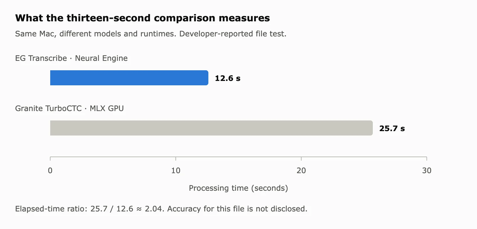
The project reports one hour processed in 12.6 seconds, with Granite TurboCTC taking 25.7 seconds on the same M3 Air. The elapsed-time difference is approximately 2.04 times. Those are developer measurements, rather than results reproduced by Perit.
Even this relatively useful comparison changes more than the recognizer. Haku reports Neural Engine execution; Granite uses an MLX GPU path. The result compares deployed systems. Isolating an architectural advantage would require additional controls over runtime and measurement boundaries.
The hour matters as much as the processor. A batch system can amortize setup costs over a long recording. Short clips expose overhead repeatedly. The audio’s difficulty also affects recognition quality, independently of how efficiently the runtime executes it.
FluidAudio’s benchmark tables make that dependence visible. On its M5 Pro setup, Parakeet v3 reaches roughly 149–152 times real time on short LibriSpeech clips and 335 times on a concatenated hour of Earnings22. The corresponding reported WER changes from 2.27% to 16.5%. The recordings are different workloads, so neither row predicts the other.
In the hour-long table, Phonon-2 reaches 480 times real time with 17.2% WER, while Parakeet Ultra reaches 457 times with 13.5%. The fastest entry is not the most accurate. None supplies the missing quality measurement for Haku’s timed file.
There is also a simple arithmetic check. Exactly 3,600 seconds divided by 12.6 is about 286 times real time. Quoting the elapsed time avoids implying that the recording’s precise duration or the timer’s boundaries are known. Model loading, resampling, segmentation, and formatting all deserve explicit treatment.
An enterprise buyer needs the paired observation: this system took this long on this recording and made these errors. A speed number detached from its output is an incomplete procurement signal.
Fast files do not make fast conversations
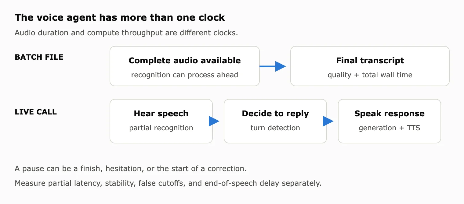
A batch recognizer receives audio that has already happened. A live assistant must wait for sound that has not happened yet. No throughput multiplier removes that constraint. Conversation adds a decision about when the available evidence is sufficient to respond.
Imagine a caller saying, “Send it to the office,” pausing, and adding, “actually, use the home address.” A system that replies during the pause may commit to the wrong destination. A system that always waits a long time avoids some interruptions but makes every exchange feel sluggish.
The relevant measurements split apart. Time to first partial text shows when recognition becomes visible. Partial stability shows how often that text changes. End-of-speech delay measures waiting after a true finish. False cutoff rate measures premature decisions. Response generation and speech synthesis contribute their own delays.
Haku’s turn-detection experiment is revealing because it encountered a training mismatch. Final, punctuated transcripts looked different from the partial text emitted during streaming. The last live partial could lag the final words. Labels that assumed the final transcript would appear were training against an unavailable observation.
After adjusting labels and using a pretrained LFM2.5-230M base with a small adapter, the reported correctly timed endings rose from 40.9% to 60.0%. Early endings remained 17.8%, and timeouts 19.1%. The evaluation replayed the full recorded corpus and tuned the threshold there; it was not a held-out production test.
The lesson is larger than the percentages. Training examples should reflect what the component will actually see at decision time. A clean final sentence and an unstable live prefix are different inputs. Better language understanding cannot repair a label that describes information the model has not received.
LiveKit’s June 2026 update tackles turn detection directly from audio, combining semantic and acoustic information. That direction highlights another limitation of text alone: hesitation, prosody, and conversational intent can matter before a final transcript exists.
A small specialist can hide a large dependency
The word “small” becomes slippery in a modular system. A reader’s trainable parameters are one quantity. Resident encoder weights, candidate vectors, temporary buffers, and application memory are others. The adaptation budget and the deployment footprint answer different questions.
The official model card separates EmbeddingGemma 2 into a 270M text component, a 170M vision encoder, and a 300M audio encoder. It also documents an 8,192-token context budget, with audio represented at about 25 tokens per second. An audio-only input therefore fits roughly 5.5 minutes.
An hour-file demo does not establish an hour-long context. Segmentation is a natural engineering explanation, but the transcriber’s exact policy needs disclosure. Windows can cut through words. Overlap can duplicate them. Silence and changes of speaker can alter the best boundary. Long-file correctness depends on stitching as well as recognition.
The vocabulary has its own potential cost. As an illustration, 229,000 vectors with 768 coordinates stored at two bytes per coordinate occupy about 351.7 MB before overhead. At 128 coordinates, the same arithmetic gives about 58.6 MB. These are examples, not measurements of Haku’s storage or reader.
Smaller vectors and fewer loaded encoders reduce different resources. Retrieval quality after embedding truncation also cannot establish transcription quality after adaptation. Every optimization must be tested at the output where its information loss matters.
The project lists a 715 MB first-run download. That does not describe active RAM, battery use, or thermal behaviour. A laptop running a recognizer beside a browser and a video call needs a different resource test from an otherwise idle machine processing one file.
The surrounding failures tell a better story
The strongest evidence for specialist architecture is often a boundary discovered in practice. Haku’s dictation formatter uses a 60M T5 model, with its encoder on the Neural Engine and decoder on the GPU. It reports typical end-to-end cleanup around 80–115 milliseconds. Its difficulties include recognizing lists without explicit cues.
Formatting is a separate obligation from recognition. Removing fillers can improve an email. The same cleanup can erase hesitation that matters in a research transcript. Haku describes leaving raw dictation untouched in terminals and code editors. The destination determines what counts as an improvement.
Its small tool-calling prototype makes the distinction sharper. The author reports roughly 98% accuracy for action, due date, and priority on novel requests, while exact title copying reaches only about 23%. Routing intent and preserving arbitrary text are separable capabilities. Correct fields do not compensate for a damaged task name.
The parallel MOSS speech-synthesis experiment exposes another measurement trap. Reported total decode time falls from 27.3 to 13.5 milliseconds per frame. Generated speech can transcribe correctly while its audible texture deteriorates. Training used only 350 sentences, and agreement in fine codebooks was low.
An automated recognizer hears enough linguistic content to recover the words. A person hears the voice. Those observations can disagree without either measurement being broken. They describe different dimensions of quality.
Together, these experiments suggest an evaluation rule for modular AI: test the handoff as well as the component. The recognizer hands words to the formatter. Partial text feeds the endpointer. Structured fields feed software. Each boundary can preserve the headline metric while losing something the next stage needs.
The baseline depends on the job
The local speech landscape already contains dedicated recognizers. IBM Granite Speech 5.0 TurboCTC is an English encoder-only CTC model. NVIDIA Parakeet TDT v3 covers 25 European languages and provides punctuation and timestamps. Qwen3-ASR supports 30 languages, including Hindi, with offline and streaming paths.
There are platform baselines, too. Apple’s SpeechAnalyzer session presents on-device transcription for live and long-form audio. Moonshine’s streaming work examines low-latency recognition as sound arrives. These systems deserve comparisons matched to the application, rather than a single ranking assembled from incompatible numbers.
Archive processing needs accurate batch output and predictable resource consumption. Dictation needs responsive text and faithful cleanup. A voice agent needs stable partials, turn decisions, and interruption handling. A multilingual support desk needs language and accent coverage that the current English-only Haku reader does not promise.
Some applications need retrieval rather than a complete transcript. DigUp uses EG2 for local search across media. The separate Linux project Recall indexes audio moments for search. Finding a discussion about a deadline can be sufficient for discovery. Quoting the deadline still requires checking the underlying evidence.
The useful comparison begins with a task description. What output will be consumed, by whom, and what mistake would make it unusable? The model shortlist follows that answer.
The evaluation should resemble the work
Start with one consented call containing ordinary speech and inconvenient details. Include an unfamiliar surname, a reference code, a corrected amount, a pause, and background noise. Keep an independently reviewed reference transcript. This is a proposed evaluation design, not a test Perit has performed on the app.
Run candidate systems on the same files and hardware. Record versions and timing boundaries. Separate cold loading from warm processing. Repeat timings, pair each file’s speed with its quality result, and retain unedited output. A repeatable comparison can remain modest in size while being honest about its scope.
Then divide the errors by mechanism. Did recognition miss an entity? Did formatting change it? Did segmentation repeat a boundary word? Did the endpoint decision discard a correction? A single final score cannot tell the team which component to change.
For streaming evaluation, save the sequence of partial transcripts with their arrival times. Annotate when the speaker truly finishes and where a pause is intentional. Test unseen speakers and sessions after choosing thresholds. Word timestamps help distinguish a recognizer that hears the phrase late from an endpointer that waits unnecessarily.
This is where Perit’s transcription and alignment method fits the argument: references should preserve the words and timing needed to score the behaviour. Fillers, false starts, overlap, and corrections are evidence of the interaction. Erasing them can make evaluation cleaner while making it less faithful to the task.
Indian English and Hinglish deserve distinct treatment. Test Indian English against the documented English capability. Label Hindi or Hinglish samples as exploratory if the reader remains English-only. A multilingual base representation does not establish multilingual recognition from a downstream English reader.
Finally, compare correction effort. Faster inference can save machine time while shifting work to reviewers. An illustrative cost model adds compute, deployment overhead, and human correction. The cheapest useful transcript is the one that meets the required quality with the lowest total effort.
Back to the hour-long recording
The 12.6-second result is worth investigating. It suggests that a broad pretrained representation can be adapted into a responsive local recognizer. It also shows why a consumer-device implementation deserves attention alongside the model architecture.
The remaining questions are concrete: which audio supports the current accuracy claim, what the timer includes, how unknown words are represented, how windows are stitched, and whether code, weights, and a benchmark harness become available. Missing disclosure defines the next experiment. It does not establish failure.
Local execution can remove a required cloud inference call from this workflow. It does not automatically establish a privacy audit, low energy use, or complete commercial readiness. Those are measurable properties of the application and deployment, with their own evidence.
The progress bar has finished. The enterprise question now lives in the transcript: did it keep “not,” preserve Kaira’s reference, and leave the correction intact? For a conversation, there is another question: did the assistant wait long enough to hear it?
Speed makes speech available. Fidelity makes it usable.
Research checked 13 October 2026. This article draws on project pages, primary research, model documentation, repositories, and the creator’s public discussion. Performance figures remain publisher-reported. Perit has not installed this app, reproduced its benchmark, or audited its network behaviour for this article. Illustrative calls, arithmetic examples, and the proposed evaluation are not collected results. Source-release and roadmap statements should be read as plans unless completed artifacts are available.